TeX (/’tɛx/tekh, often pronounced TeK in English) is a very widespread and popular way of representing Mathematics notation using only characters that you can type on a keyboard. This makes it a useful format to use in LMS since it can be entered anywhere you can type text, from forum posts to quiz questions.

TeX expressions can be entered in multiple ways:

• typing them directly into texts.
• using the Java-based Dragmath editor in LMS’s TinyMCE editor.
• using the HTML-based equation editor in LMS’s Atto editor

Afterward, TeX expressions are rendered into Mathematics notation:

• using the TeX filter in LMS, which uses a TeX binary installed on the server to convert expressions into .gif images (or if that is not available, it falls back to a simple built-in mimetex binary).
• using the MathJax_filter which identifies TeX expressions and uses the Mathjax JS library to render them in browsers at display time.
• using other third-party solutions.

As you can imagine, the whole field is not as simple as we would like, especially because there are many flavors of TeX and slight variations between tools.

This page focusses only on using TeX in core LMS. See the links at the bottom of this page for more information on setting up TeX editors and filters, including other tools from the LMS community that may be suitable for advanced users.

WARNING: This Wiki environment uses a DIFFERENT TeX renderer to LMS, especially when it comes to controlling sequences. For this reason, images are sometimes used to represent what it should look like in LMS. YMMV.

Language Conventions

To identify a TeX sequence in your text, surround it with $$ markers. To invoke a particular command or control sequence, use the backslash, A typical control sequence looks like:

 $$ x = frac{sqrt{144}}{2} times (y + 12) $$  

Additional spaces can be placed into the equation using the without a trailing character.

Equation displayed on its own line

When an equation is surrounded by a pair of $$ markers, it is displayed centered on its own line. The $$’s are primitive TeX markers. With LaTeX, it is often recommended to use the pair [ and ] to enclose equations, rather than the $$ markers, because the newer syntax checks for mistyped equations and better adjust vertical spacing. If the TeX Notation filter is activated, which set a LaTeX renderer, the same equation as above is obtained with the following control sequence:

 [ x = frac{sqrt{144}}{2} times (y + 12) ]

However, if the equation is mistyped, it will be displayed enclosed in a box to signal the mistake and if the equation appears in a new paragraph, the vertical space above the equation will adjust correctly.

Using [ … ] instead of $$ … $$ may have other advantages. For example, with the Wiris equation editor installed, the Atto editor undesirably transforms the TeX code of equations enclosed with $$ into XML code, whereas it does not do so when the equations are enclosed with [ and ].

 

Equation displayed within text

With the TeX notation filter activated, an equation is displayed within the text when it is surrounded by the pair ( and ). For example, the following:

 The point ( left( {{x}_{0}}+frac{1}{pleft( {{x}_{0}} right)} , frac{qleft( {{x}_{0}} right)}{pleft( {{x}_{0}} right)} right) ) is located...

will display as follows:

Note that the single $ marks may not work for this purpose.

Reserved Characters and Keywords

Most characters and numbers on the keyboard can be used at their default value. As with any computing language, though, there are a set of reserved characters and keywords that are used by the program for its own purposes. TeX Notation is no different, but it does have a very small set of Reserved Characters. This will not be a complete list of reserved characters, but some of these are:

 @ # $ % ^ & * ( ) . 

To use these characters in an equation just place them in front of them like $ or %. If you want to use the backslash, just use a backslash. The only exception here seems to be the &, ampersand.

 

Superscripts, Subscripts, and Roots

Superscripts are recorded using the caret, ^, symbol. An example of a Maths class might be:

 $$ 4^2  times  4^3  = 4^5 $$
 This is a shorthand way of saying: 
 (4 x 4) x (4 x 4 x 4) = (4 x 4 x 4 x 4 x 4)
 or
 16 x 64 = 1024.
 

Subscripts are similar but use the underscore character.

 $$ 3x_2  times  2x_3 $$
 
 

This is OK if you want superscripts or subscripts, but square roots are a little different. This uses a control sequence.

 $$ sqrt{64}  =  8 $$
 
 

You can also take this a little further, but adding in a control character. You may ask a question like:

 $$ If  sqrt[n]{1024}  =  4,  what  is  the  value  of  n? $$  
 

Using these different commands allows you to develop equations like:

 $$ The sqrt{64}  times  2  times  4^3  =  1024 $$
 
 

Superscripts, Subscripts, and roots can also be noted in Matrices.

Fractions

Fractions in TeX are actually simple, as long as you remember the rules.

 $$ frac{numerator}{denominator} $$ which produces 

This can be given as:

This is entered as:

 $$ frac{5}{10}  is  equal  to  frac{1}{2}.$$

With fractions (as with other commands) the curly brackets can be nested so that for example you can implement negative exponents in fractions. As you can see,

 $$frac {5^{-2}}{3}$$ will produce 

 $$left(frac{3}{4}right)^{-3}$$ will produce   and

 $$frac{3}{4^{-3}}$$ will produce 

 You likely do not want to use $$frac{3}{4}^{-3}$$ as it produces 

You can also use fractions and negative exponents in Matrices.

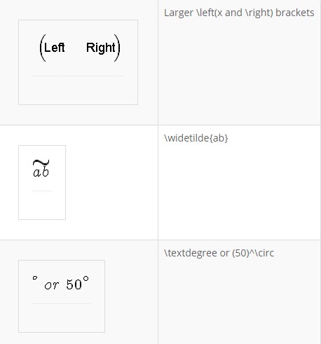
Brackets

As users advance through Maths, they come into contact with brackets. Algebraic notation depends heavily on brackets. The usual keyboard values of ( and ) are useful, for example:

he is written as:

 $$ d = 2 \ \ times \ (4 \  -  \j) $$

Usually, these brackets are enough for most formulae but they will not be in some circumstances. Consider this:

Is OK, but try it this way:

This can be achieved by:

 $$ 4x^3  +  left(x  +  frac{42}{1 + x^4}right) $$

A simple change using the left( and right) symbols instead. Note the actual bracket is both named and presented. Brackets are almost essential in Matrices.

Ellipsis

The Ellipsis is a simple code:

Written like:

 $$ x_1,  x_2,  ldots,  x_n  $$

A more practical application could be:

Question:

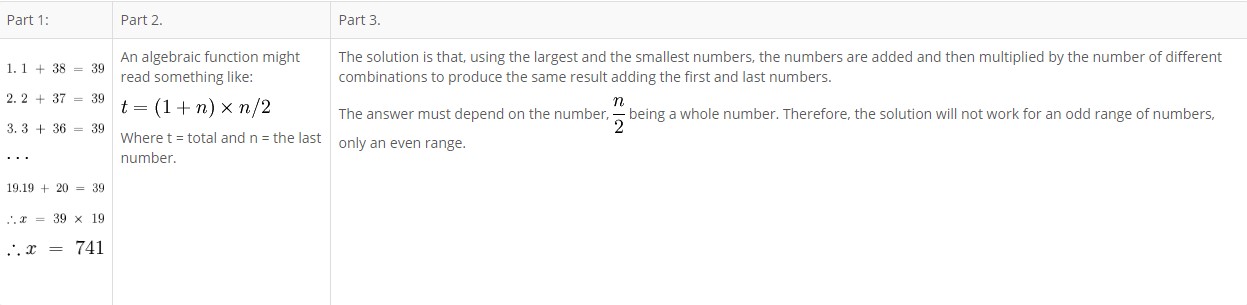
 "Add together all the numbers from 1........ 38.
 What is an elegant and simple solution to this problem?
 Can you create an algebraic function to explain this solution?
 Will your solution work for all numbers?"

Answer:
The question uses an even number to demonstrate a mathematical process and generate an algebraic formula.

 

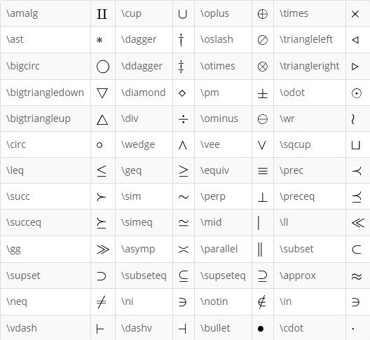
Symbols

These are not all the symbols that may be available in TeX Notation for LMS, just the ones that I have found to work in LMS.

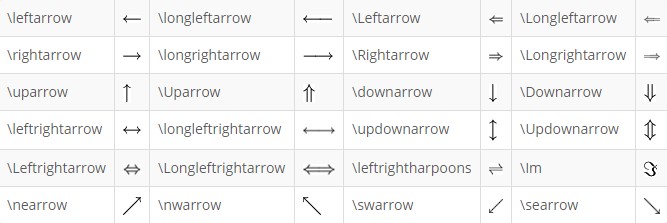
Arrows

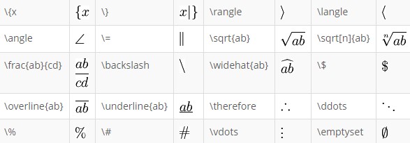
Delimiters and Maths Constructs

NOTE: Most delimiters and constructs need additional parameters for them to appear appropriately.

WARNINGS: The & character in LaTeX usually requires a backslash, In TeX Notation for LMS, apparently, it does not. Other packages, AsciiMath, may use it differently again so be careful using it. The copyright character may use the MimeTeX charset and produces a copyright notice for John Forkosh Associates who provided a lot of the essential packages for the TeX Notation for LMS, so I understand. I have been, almost reliably, informed that a particular instruction will produce a different notice though .:)

There are also a number of characters that can be used in TeX Notation for LMS but do not render in this page:

Greek Letters

Notable Exceptions

Greek letter omicron (traditionally, mathematicians don’t make much use of omicron due to possible confusion with zero). Simply put, lowercase omicron is an “o” rendered as o. But note omicron may now work with recent TeX implementations including MathJax.

At the time of writing, these Greek capital letters cannot be rendered by TeX Notation in LMS:

Alpha, Beta, Zeta, Eta, Tau, Chi, Mu, Iota, Kappa and Epsilon.

TeX mathematics adopts the convention that lowercase Greek symbols are displayed as italics whereas uppercase Greek symbols are displayed as upright characters. Therefore, the missing Greek capital letters can simply be represented by the mathrm{ } equivalent

Boolean algebra

There are a number of different conventions for representing Boolean (logic) algebra. Common conventions used in computer science and electronics are detailed below:

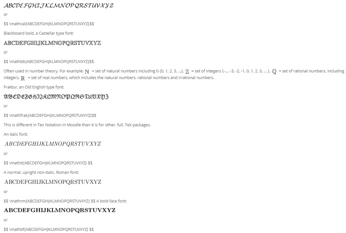
Fonts

To use a particular font you need to access the font using the same syntax as demonstrated above.

A math calligraphic font:

Size of displays

The default size is rendered slightly larger than normal font size. TeX Notation in LMS uses eight different sizes ranging from “tiny” to “huge”. However, these values seem to mean different things and are, I suspect, dependent upon the User’s screen resolution. The sizes can be noted in four different ways:

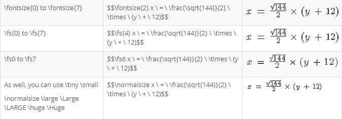
It appears that TeX Notation in LMS now allows fs6, fs7, huge and Huge to be properly rendered.

Color

Unlike many scripting languages, we only need to name the colour we want to use. You may have to experiment a little with colors, but it will make for a brighter page. Once named, the entire statement will appear in the color, and if you mix colors, the last named color will dominate. Some examples:

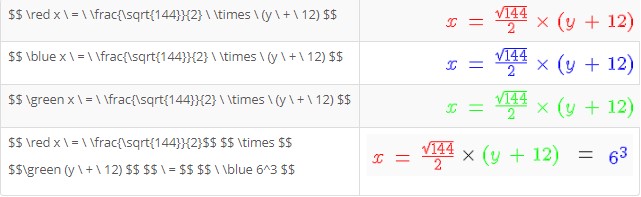
LMS note: You may find this doesn’t work for you. You can try to add “usepackage{color}” to your tex notation setting “LaTeX preamble” (under Site adminstration/Plugins/Filters/TeX notation)and then use this new syntax: $$ color{red} x = frac{sqrt{144}}{2} times (y + 12) $$

You may note this last one, it is considerably more complex than the previous for colours. TeX Notation in Windows does not allow multicoloured equations, if you name a number of colours in the equation, only the last named will be used.

Geometric Shapes

There are two ways to produce geometric shapes, one is with circles and the other is with lines. Each take a bit of practice to get right, but they can provide some simple geometry. It may be easier to produce the shapes in Illustrator or Paint Shop Pro or any one of a number of other drawing packages and use them to illustrate your lessons, but sometimes, some simple diagrams in LMS will do a better job.

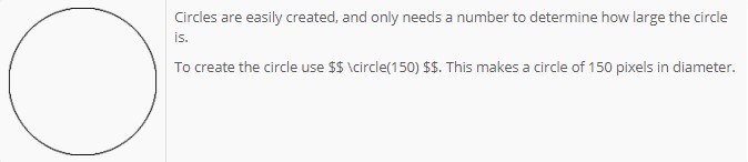
Circles

Circles are easy to make.

Creating Arcs

Arcs are also easy to produce, but require some additional parameters. The same code structure used in circles create the basic shape, but the inclusion of a start and end point creates only the arc. However, notice where the 0 point is, not at the true North, but rather the East and run in an anti-clockwise direction.

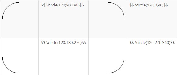
This structure breaks down into the circle command followed by the diameter, not the radius, of the circle, followed by a semi-colon, then the demarcation of the arc, the nomination of the start and end points in degrees from the 0, East, start point. Note that the canvas is the size of the diameter nominated by the circle’s parameters.

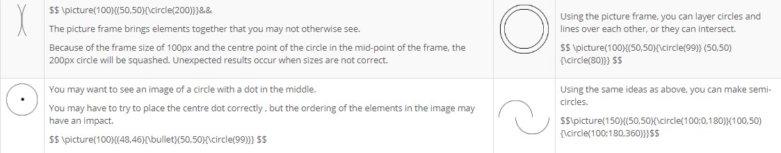
The picture Command

Using circles and arcs as shown above is somewhat limiting. The picture command allows you to use a frame in which to build a picture of many layers. Each part of the picture though needs to be in its own space, and while this frame allows you to be creative, to a degree, there are some very hard and fast rules about using it.

All elements of a picture need to be located within the picture frame. Unexpected results occur when parts of an arc, for example, runs over the border of the frame. (This is particularly true of lines, which we will get to next, and the consequences of that overstepping of the border can cause serious problems.)

The picture command is structured like:

  picture(100){(50,50){circle(200)}}
  command(size of frame){(x co-ordinate, y co-ordinate){shape to draw(size or x co-ordinate, y co-ordinate)})  

NOTE: The brace is used to enclose each set of required starting point coordinates. Inside each set of braces, another set of braces is used to isolate each set of coordinates from the other, and those coordinates use their proper brackets and backslash. Count the opening and closing brackets, be careful of the position,

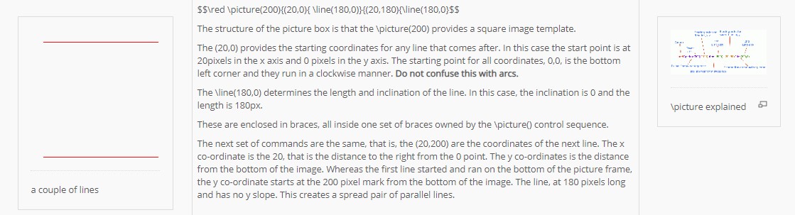
Lines

---

Warning: Drawing lines in TeX Notation in LMS is an issue, go to the Using Text Notation for more information. If the line is not noted properly then the parser will try to correctly draw the line but will not successfully complete it. This means that every image that needs be drawn will be drawn until it hits the error. When the error is being converted, it fails, so no subsequent image is drawn. Be careful and make sure your line works BEFORE you move to the next problem or next image.

---

While this explains the structure of a line, there is a couple of elements that you need to go through to do more with them.

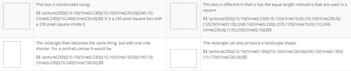
Squares and Rectangles

Drawing squares and rectangles is similar, but only slightly different.

There should be a square box tool, and there is, but unless it has something inside it, it does not display. It is actually easier to make a square using the line command.

Controlling Angles

Controlling angles is a little different. They involve a different perception, but not one that is unfamiliar. Consider this:

We have a point from which we want to draw a line that is on an angle. The notation used at this point can be positive, positive or positive, negative or negative, positive or negative, negative. Think of it like a number plane or a graph, using directed numbers. The 0,0 point is in the center, and we have four quadrants around it that give us one of the previously mentioned results.

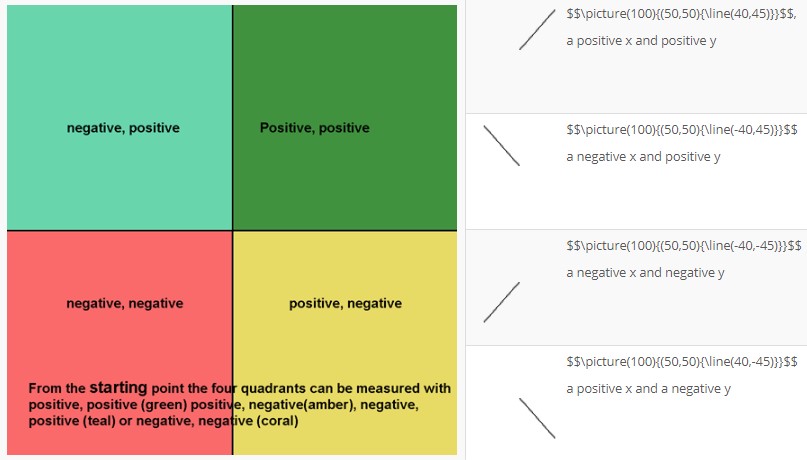
Essentially, what these points boil down to is that anything above the insertion point is positive on the y-axis, anything below is negative. Anything to the left of the insertion point is negative while everything to the right is positive.

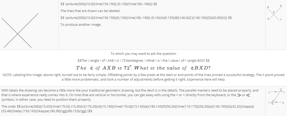
Intersecting Lines

You can set up an intersecting pair easily enough, using the picture control sequence.

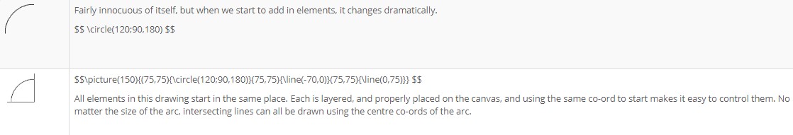
Lines and Arcs

Combining lines and arcs is a serious challenge actually, on a number of levels. For example, let’s take an arc from the first page on circles.

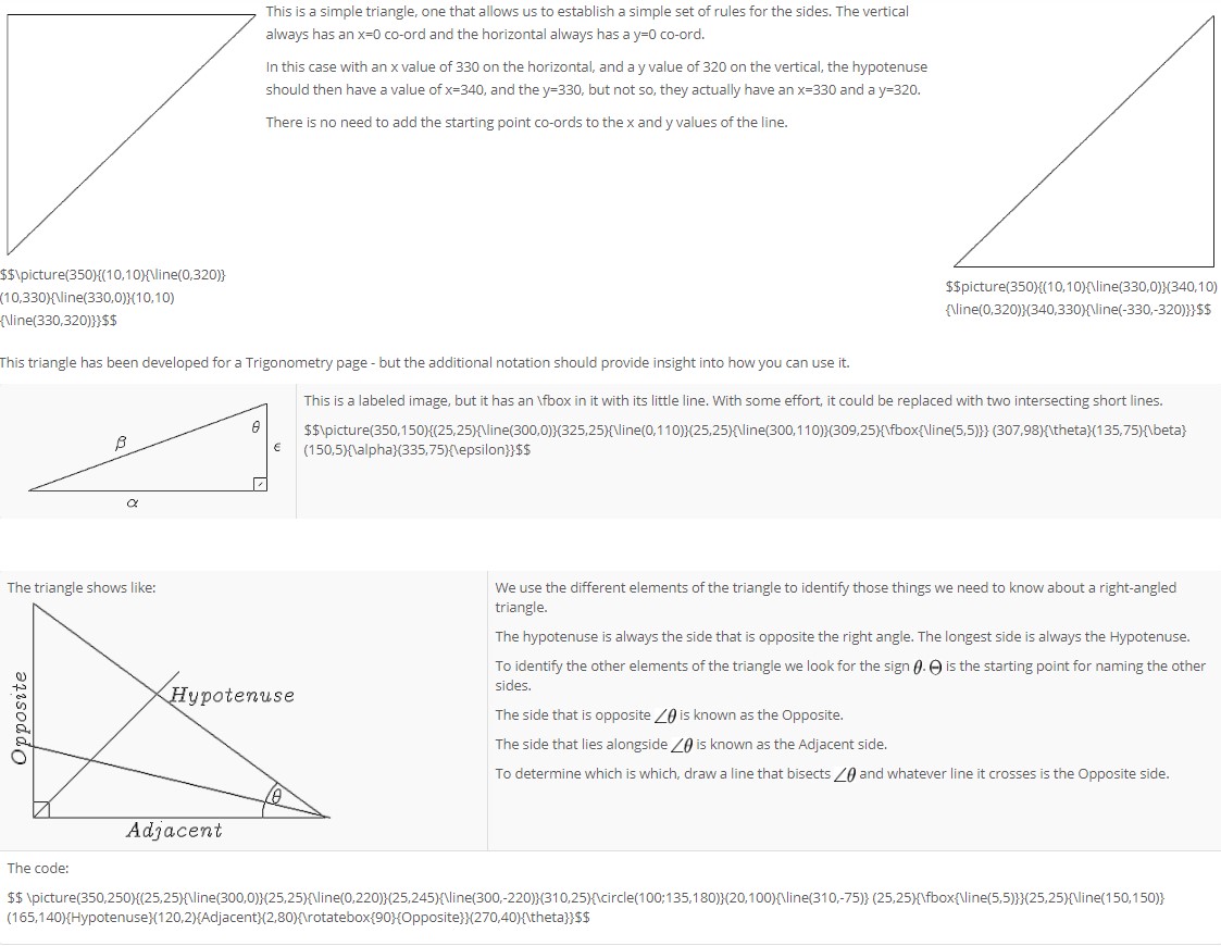
Triangles

Of all the drawing objects, it is actually triangles that present the most challenge. For example:

 

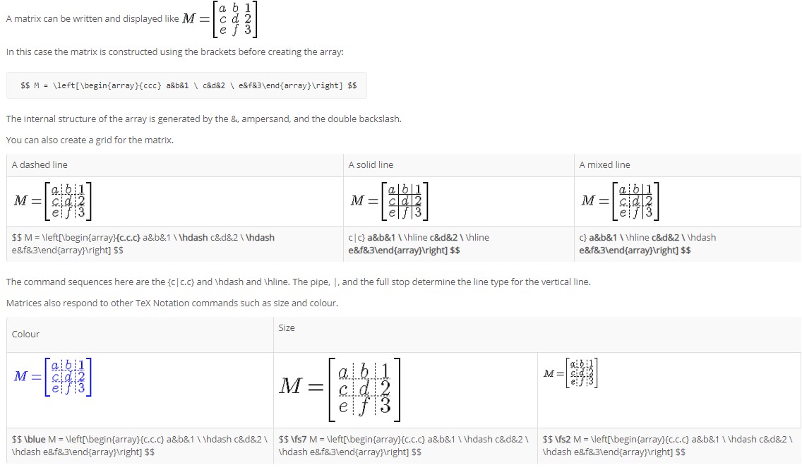
Matrices

A Matrix is a rectangular array of numbers arranged in rows and columns which can be used to organize numeric information. Matrices can be used to predict trends and outcomes in real situations – i.e. polling.

 

A Matrix

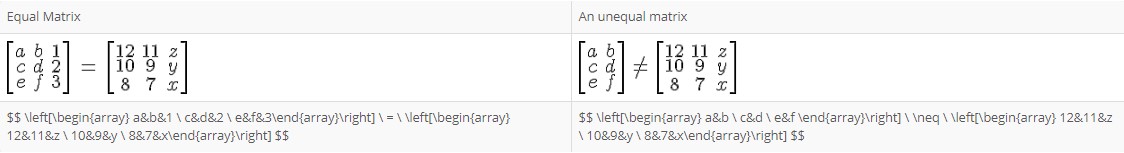
Creating equal and unequal matrices

Equal and unequal matrices are simply matrices that either share or not share the same number of rows and columns. To be more precise, equal matrices share the same order and each element in the corresponding positions are equal. Anything else is unequal matrices.

Actually equal and unequal matrices are constructed along similar lines, but have different shapes:

Labeling a Matrix

Addition and subtraction matrices are similar again, but the presentation is usually very different. The problem comes when trying to mix labels into arrays. The lack of sophistication in the TeX Notation plays against it here.

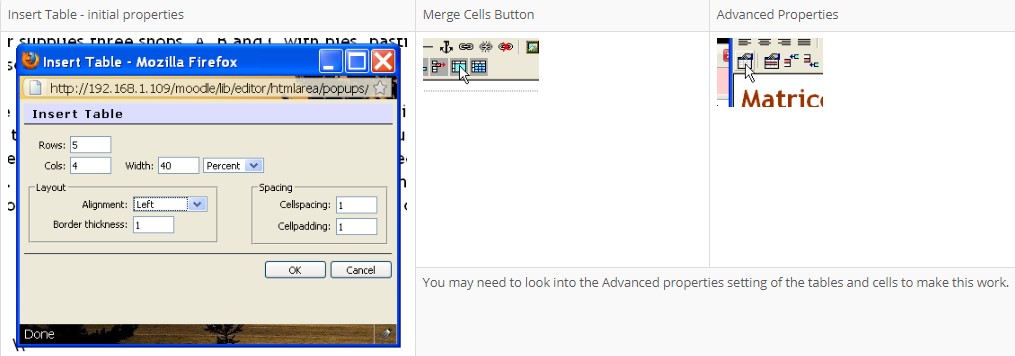
LMS allows an easy adoption of tables to make it work though. For example:

 Bill the baker supplies three shops, A, B and C with pies, pasties and sausage rolls. 
 He is expected to determine the stock levels of those three shops in his estimation of supplies.

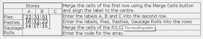
It is better to use the LMS Fullscreen editor for this, to have a better idea of how the end product will look and to take advantage of the additional tools available. Design decisions need to occupy our attention for a while. We need a table of five rows and four columns. The first row is a header row, so the label is centred. The next row needs four columns, a blank cell to start and labels A, B and C. The next three rows are divided into two columns, with the labels, pies, pasties and sausage rolls in each row of the first column and the matrix resides in a merged set of columns there. So first the table:

This is the immediate result:

While not a very good look, it can be made better by tweaking the table using the advanced settings and properties buttons and then you can tweak the matrix itself.

Tweaking the Matrix

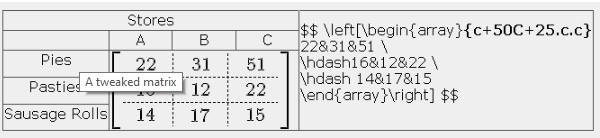
Things are not always as they seem, be aware, the “c” does not stand for “column”, it actually stands for “centre”. The columns are aligned by the letters l, for the left, c for centre and r for the right.

Each column is spread across 50 pixels, so the value of 50 is entered into the alignment declaration. The plus sign before the value is used to “propogate” or to force the value across the whole matrix, but is not used when wanting to separate only one column.

To set the rows is a little more problematic. The capital letter C sets the vertical alignment to the centre, (B is for baseline, but that does not guarantee that the numbers will appear on the base line, and there does not appear to be any third value). The plus sign and following value sets the height of all rows to the number given. In this, I have given it a value of 25 pixels for the entire matrix. If there were four or five rows, the same height requirement is made.

The order things appear is also important. If you change the order of these settings, they will either not work at all, or will not render as you expect them to. If something does not work properly, then check to make sure you have the right order first.

An Addition Matrix

The rule for performing operations on matrices is that they must be equal matrices. For example, addition matrices look like:

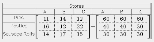
with the results obvious. The code is:

 $$left[begin{array}{c+50C+25.c.c}
 11&14&12  hdash16&12&22  hdash 14&17&15
 end{array}right] + left[begin{array}{c+50C+25.c.c}
 60&60&60  hdash 40&40&30  hdash 30&30&30
 end{array}right] $$

A Subtraction Matrix

Similar to an addition matrix in its construction, the subtraction matrix is subject to the same rules of equality.

Using the same essential data, we can calculate the daily sales of each of the shops.

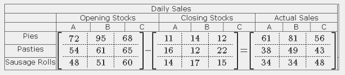
The code is:

 $$ left[begin{array}{c+50C+25.c.c}
 72&95&68  hdash 54&61&65  hdash 48&51&60
 end{array}right] - left[begin{array}{c+50C+25.c.c}
 11&14&12  hdash 16&12&22  hdash 14&17&15
 end{array}right] = left[begin{array}{c+50C+25.c.c}
 61&81&56  hdash 38&49&43  hdash 34&34&48
 end{array}right] $$  

This code looks more complex than it really is, it is cluttered by the lines and alignment sequences.

Multiplication Matrices

Different than the addition or subtraction matrices, the multiplication matrix comes in three parts, the row matrix, the column matrix and the answer matrix. This implies it has a different construction methodology.

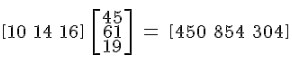
And the code for this is:

 $$ begin{array} 10&14&16end{array}  
 left[begin{array} 45 \ 61 \ 19 end{array}right] 
  =  begin{array} 450&854&304end{array} $$

While different, it is not necessarily more complex. For example a problem like:

 Bill the baker is selling his product to Con the cafe owner, who 
 wants to make sure his overall prices are profitable for himself. 
 Con needs to make sure that his average price is providing sufficient 
 profit to be able to keep the cafes open. Con makes his calculations 
 on a weekly basis, comparing cost to sale prices.

With the pies, pasties and sausage rolls in that order he applies them to the cost and sale price columns :

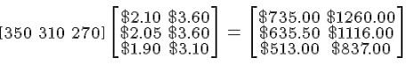
The code for this is:

 $$left[begin{array} 350&310&270 end{array}right]  
 left[begin{array} $2.10&$3.60  $2.05&$3.60  $1.90&$3.10 end{array} 
 right]  =  left[begin{array} $735.00&$1260.00  $635.50&$1116.00  
 $513.00&$837.00 end{array}right] $$